Determining which Fantasy Premier League models are good, bad or middling isn’t totally obvious at first glance and getting a feel for what a perfect model may look like is seemingly even more abstract to our minds.
In this article I will share high level information on the approach used to create “Perfect model” conditions and what we can take away from it’s performance relative to real world models, having been inspired by @mmreyno. Data for these models for the 22/23 season to date (for period between GW1 to GW21) has kindly been shared by @sertalpbilal.
I also have included a reference to the performance of xG models too and give some perspective on ensemble models.
The Ultimate Truth Model
In reality a “Perfect”/”Ultimate Truth” model would reflect the true likelihoods and forecast of the future at a given point in time, rather than mere estimates or gut feelings. In the context of FPL this would be having perfect information at deadline time (or maybe 15 minutes before in case the server crashes). This level of knowledge is clearly impossible, however there is a perspective that allows for what this would look like to be estimated.
As part of the fplreview.com site 1,000 simulations of each players performance every GW are performed. Each match is simulated with players scoring goals, winning clean sheets, being substituted and even being awarded bonus etc. this is powered by evaluations made by the Massive Data model. These simulations are also used to produce some of the insights and visuals in the Season Review/Gameweek Analysis tools.
The plot below illustrates what these simulations look like (and what EV actually represents), a wide array of diverse outcomes for Kane/Haaland in GW21.
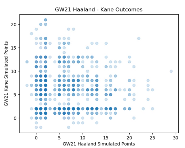
In this simulation dataset we have perfect information. “True EV” is the average value across all simulations. Each individual simulation represents the outcome in a world. By comparing the “True EV” to the outcome in each world using model accuracy metrics we can develop an understanding of how a perfect model may perform.
Of course it must be stated that no truly perfect simulation of the game can exist, but certainly for this context it will help produce very useful benchmark.
Measuring Model Accuracy
Three commonly used metrics have been applied in this analysis to determine projection accuracy:
- Root Mean Square Error (RMSE) Lower is better
- Mean Absolute Error (MAE) Lower is better
- Coefficient of Determination (R2) Higher is better
In simpler terms the projection (EV) for each GW is compared to the outcome (FPL points) each GW and is assessed based on the metrics above.
To determine the predictions from the perfect model that can be compared to existing models, I found “in-common” EV predictions across the 6 real world models provided- totalling 3,730 samples. I then analysed how well the “Perfect Model” performed in each of the 1,000 simulated worlds.

As we can see there’s variation in how a perfect model may perform- depending on how crazy/unexpected the results are. The R2 scores may be lower than many might expect, but in reality this is a reflection of the scale of variance in FPL and there’s just no avoiding that, sadly.
Notably, this ceiling in predictive performance doesn’t just apply to models- it applies to any human capability to predict FPL points, nobody can escape what is a pretty hard limitation over enough samples.
From the perspective of a modeller, each step towards the ceiling becomes increasingly more difficult- before an effective plateau is reached. We can’t ever achieve a perfect model, but how good are the ones we can create?
How do Real World FPL Models Compare?
As described earlier, 6 FPL projection models with 3,730 common predictions from GW1-21 have been identified. The performance of the projections made by these models is once more measured by RMSE, R2 and MAE, which can be directly compared with how a perfect model has been estimated to perform over the same sample and metrics. Results are visualised and tabulated below:

| Model | RMSE | MAE | R2 |
| Simulated “Perfect Model” | ~2.7-2.9 | ~1.9-2.0 | ~0.12-0.17 |
| fplreview MD Model | 2.803 | 1.973 | 0.151 |
| Model B | 2.816 | 2.020 | 0.143 |
| Model C | 2.829 | 1.995 | 0.136 |
| Model D | 2.843 | 2.059 | 0.127 |
| Model E | 2.852 | 2.011 | 0.121 |
| Model F | 2.884 | 2.115 | 0.102 |
| All Players 2.7EV | 3.043 | 2.239 | 0.000 |
Interestingly, the best current models are performing at levels within the realm of what we might see from a perfect model, which may be surprising (not to suggest that any perfect models exist or will ever exist). It may be fair to say that periodic variance has helped a little, indeed there is a pretty wide variation in perfect model performance depending on how predictable events in a period is, and also that this simulation itself can never truly be perfect, though it’s a powerful reference point.
Overall the models that the community has generally understood to be the best/worst are largely (and unsurprisingly) agreeing with the reality described in the data. If you are struggling to interpret the data, it’s definitely a very positive result for the Massive Data model- having the lowest RMSE, MAE and highest R2 across the natural models.
Lessons from xG Models
Even understanding what the ceiling for projections may look like, it has to be appreciated that those RMSE, MAE and R2 values don’t really offer much scale or sense of difference. To help understand this better, I am going to lean on a dataset that is now more widely understood in football, xG, and determine how a great model that aligns pretty well with human eyes, compares to a pretty crude model and also just assuming every shot has an equal chance of going in.
The same performance metrics are applied to xG for the “Big 5” leagues in Europe so far in the 2022/2023 season.
| Model | RMSE | MAE | R2 |
| Gold Standard xG | 0.276 | 0.153 | 0.212 |
| Crude xG | 0.283 | 0.162 | 0.169 |
| Every shot is 0.11 xG | 0.311 | 0.194 | 0.000 |
It may be hard to tell, but in reality that is a resounding gap in performance between a gold standard xG model and something very crudely put together. Looking at clips of various chances and the xG awarded by both models makes the gap in quality even more obvious, however there’s no real need to go to that level of detail. What’s more, the gap in accuracy metrics is of a proportional scale that helps us understand the gap within FPL projection models.
Ensemble Models
Something that is worthy of consideration is the concept of Ensemble models (more info here). In simple terms this is combining data from several independent models into one model, similar to the kind of value we find in the “wisdom of the crowd” idea.
So given this concept, let’s test out three pretty simple interpretations of what an ensemble model may look like, and how it might perform
- “Average Ensemble”: The average prediction across all models
- “User Weighted Ensemble”: There’s a pretty strong consensus that all models are likely indeed not equal. Weighing 3 popular models within analytics circles at 60:30:10 would seem reasonable.
- “Linear Regression: Weighted Ensemble”: Using GW1-12 data as training data to determine weighting coefficients in each model through linear regression. This trained model is then applied to GW13-21 test data (to avoid over-fit results).
| Model | RMSE | MAE | R2 |
| Simulated “Perfect Model” | ~2.7-2.9 | ~1.9-2.0 | ~0.11-0.19 |
| fplreview MD Model | 2.830 | 2.009 | 0.148 |
| Model B | 2.859 | 2.061 | 0.130 |
| Model C | 2.872 | 2.039 | 0.122 |
| Model D | 2.883 | 2.104 | 0.115 |
| Model E | 2.877 | 2.044 | 0.119 |
| Model F | 2.923 | 2.141 | 0.091 |
| “Average Ensemble” | 2.835 | 2.030 | 0.145 |
| “User Weighted Ensemble” | 2.830 | 2.019 | 0.148 |
| “Regression Ensemble” | 2.842 | 2.048 | 0.140 |
The ensemble models end up doing well compared to many other models. The ability to dampen out mistakes in individual models holds value, though equally sometimes it can potentially come at the cost of special insights too. I would suggest the gaps between the different ensemble models are so slim that it shouldn’t be taken as evidence of one approach being better than another, there are many considerations needed.
With enough data, different regression approaches should be extremely useful to use as a starting point. Conversely, models tend to develop over time and new models pop up, thus giving weight to our own belief/insights on the models is not a terrible idea- this can fall under the realm of Bayesian thinking.
I would also suggest that we can do better than just weighing all models equally. The fact is what some models add in normalising effect, will not be worth the increased errors they also inject, equally focusing on a lower amount of models eases the level and complexity of data handling which is never fun and often a cause of its own issues.
The above is really my practical perspective on how I might go about this in simple terms- more thought, depth and certainly advanced modelling can go into ensemble modelling than this.
Conclusion
Overall, I hope this adds perspective when trying to understand projection model performance, and add a sense of scale for how the different models compare. The insights into what “perfect” modelling may look like has been fun to walk through and probably gives a hint that even if an “Ultimate Truth” model ever somehow existed, hindsight would still make it “appear” foolish.
From a fplreview.com perspective, the performance is extremely positive and the outcomes are also repeated for EV as a predictor of xG pts in the dataset too, which adds further confidence. I would also like to give credit to another excellent model out there, up to the creator if they wish to lose anonymity, of course!
It does have to be reiterated that FPL is a game that we have limited control over, and nobody/nothing can provide the outcome guarantees we’d like (outside of match fixing). Variance in the game has been understood to be high for years and this is reflected in what we can expect even a perfect model to achieve on a weekly basis, thus the only way to approach FPL is with a light grip and the occasional punt on Saint-Maximin to finally come good.
Lastly, I will always suggest a blend between models and human information is probably the most powerful (and fun) way to approach this game- solvers using model data are excellent for idea generation and offer us a chance to overlay our beliefs and intangibles, rather than necessarily getting lost in a marginally top solve.
Notes
- 1GW ahead projections are included in this dataset, however other datasets with 5+GW projections are achieving similar results
- Model dataset is not mine to share
- Accuracy metrics determined using scikit-learn python package