Shot-based xG data is becoming more mainstream and referred to more often in football circles than previously. It has the advantage over basic shot /goal data in that it gives each chance a convertibility rating- effectively adding a useful context to shot data.
Of course it gets criticism from many as it never picks up events such as a great run that wasn’t spotted by a team-mate on the day or a player failing to round the keeper instead of shooting which puts a limit on it’s capabilities- but that really should not be expected of shot-level xG data. Overall xG is an excellent descriptor of shot quality and that’s what it is designed to be.
In terms of assessing a player often xG data over a certain time period is referred to as a means of estimating a players goal-scoring potential. For a game like FPL that can have a huge amount of value- knowing a players goalscoring potential simply helps us make better and less biased decisions. Perhaps a player has high or low xG over the last 5 or 10 games, but can we draw much from this? And if not, then at what point can we finally feel confident that a players xG90 data reflects his true goalscoring potential?
In this post I aim to analyse the value of player level xG data and determine how much data is required to attain a useful indicator of goalscoring potential by creating a simulated match & xG environment.
Contents
Creating a Player Level Model
Step 1- Player Creation:
- Create player with a true goalscoring potential ([E]G90) of 0.30. This means over enough simulations the player will average 0.30 goals/match and would have been at around the level of Dele Alli or Diogo Jota. We want to see how well different time-periods of xG & actual goal data can reflect this players known ability.
Step 2- Load xG Chance Distribution:
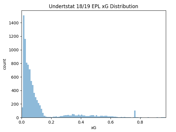
- For this analysis lets assume the player gets a normal chance quality distribution (not biased towards taking difficult or easy shots). For this I’m using the full 2018/2019 EPL Understat chance dataset as the players pool of chances.
Step 3- Calculate Average Shots per Game:
- The average amount of shots the player takes per match ([E]SH90) can be calculated from dividing his [E]G90 potential by the average xG level in his typical chance distribution. In this case is 0.30/0.1146 = 2.618. This means on average the player will take 2.618 shots per match.
Step 4- Use Poisson Distribution for Shot Data:
- We assume the players shot distribution at a match level is a Poisson distribution built from this [E]SH90 level, which is detailed in the table below for a player with an [E]SH90 level of 2.618.
| No. Shots | 0 | 1 | 2 | 3 | 4 | 5 | 6+ |
| Probability | 7.3% | 19.1% | 25.0% | 21.8% | 14.3% | 7.5% | 5.0% |
Simulating a Match (& 100,000 others)
Step 1- Generate Match Specific Shots:
- The first step in the simulation is randomly generate the number of shots given the [E]SH90 level and assuming a Poisson distribution as described above.
- Let’s say that in this example the random number generator produces 3 shots.
Step 2- Generate xG for each chance:
- Next we randomly pick the quality of the chances from the Understat EPL 2018/19 chance data.
- For the example the random number generator determines that the 3 chances have xGs of [0.03,0.15,0.32]- with a total xG of 0.50 for this simulated match.
Step 3- Generate Chance Conversion:
- Finally we use another random number generator to determine the conversion of the chances- this is applied to each shot the player took. For the [0.03,0.15,0.32] chance set there is a 56.1% chance of 0 goals, 38.0% chance of 1 goal, 5.8% chance of 2 goals and a 0.1% chance of 3 goals.
- For this example let’s say the player failed to convert all 3 chances and scored 0 goals.
Summary:
- Effectively we have simulated a match where our player with a known [E]G90 potential of 0.30 has taken 3 shots, with an xG of 0.50 but scored 0 goals.
- This match simulation is then repeated 100,000 times using a Python script to get an ultra high sample to read from and get high confidence results and it is also repeated for different fixed [E]G90 potentials for further analysis.
Analysing the Results
How Much Can We Read Into the Last 5 Matches Data?
The key aspect of this analysis is that it opens up the capability to see how much unpredictable variance impacts the data over set periods of time. Often people look at the last 5 matches as a reference, with xG data is that enough time for things to settle down?
To do this we can check how well the xG90 & G90 readings match the known [E]G90 potential over 20,000 distinct 5 match sequences from the 100,000 match sample. This is basically reviewing how worthwhile looking at last 5 match xG and goal data really is.
The histograms below display how often the same 0.30[E]G90 player would get certain xG90 and G90 ratings over a 5 match period. For example in ~350 (1.75%) of the 20,000 simulations we would see a xG90 of 0.40, in ~550 (2.75%) we would see a xG90 of 0.30 and in ~100 (0.5%) we would see an xG90 of 0.60 etc. In terms of basic goal data around 22.5% of the time the player would score 0 goals though 12.5% of the time he would be ‘on-fire’ and score 3 goals over the same 5 matches- there was an instance where he went on to score a whopping 8 goals!

Samples within 10% Precision (0.275-0.325): 15.7%
Samples within 25% Precision (0.225-0.375): 38.1%
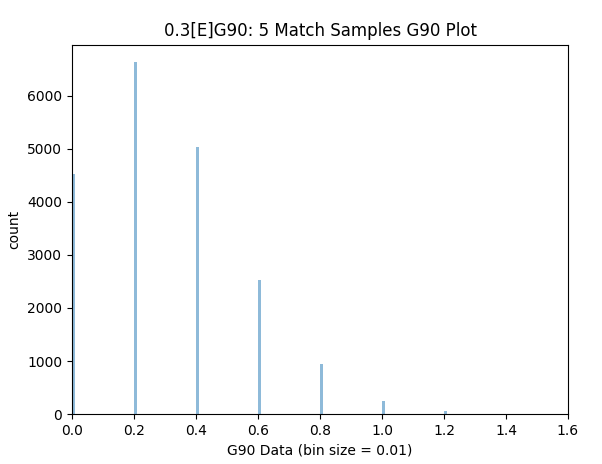
No samples can get close to 0.30 as divisor is 5
From the simulations we can see that 5 matches simply provides an ineffective amount of background data for each of these metrics and generally leads to a imprecise reading in isolation. We know that the players true goalscoring potential ([E]G90) was 0.30, but more often than not if we look a the last 5 matches we will think that it was less than 0.20 or greater than 0.40 whether we use basic goal data or even xG. This means that we will often think the player is performing well/badly if we look at the data but in reality his goalscoring potential has been totally consistent and normal and we are falling victim to unpredictable variance.
It is extremely important to note that the variance in this simulation is not due to any change in the players form/ability, his team or the opposition. Effectively the same match is being simulated 100,000 times with identical player expected pre-match goal levels. The distortion is purely due to unpredictable variance that is experienced using xG and basic goal data. Indeed this helps explain why something as subtle, fleeting and hard to pin down as form does not appear in other analysis of goalscoring data (it would simply be masked by the massive variance).
How Many Matches to Get a Useful Indicator?
So if 5 matches is imprecise- how much data do we need for worthwhile precision? Well using the same methodology distinct 10, 20, 40 & 100 match periods can be investigated. I repeated the analyses for these match periods and calculated the Mean Absolute Error (MAE), Root Mean Square Error (RMSE) & how often a reading within 10% & 25% Precision of the players actual [E]G90 potential is achieved. This is shown below in table form using simulated goal and xG data.
| xG90 Data | ||||
| Matches | MAE | RMSE | 10% Precision Achieved | 25% Precision Achieved |
| 1 | 0.255 (85%) | 0.328 | 4.0% | 10.9% |
| 5 | 0.116 (38.7%) | 0.145 | 15.7% | 38.1% |
| 10 | 0.0827 (27.6%) | 0.104 | 22.5% | 54.3% |
| 20 | 0.057 (19%) | 0.072 | 31.7% | 70.1% |
| 40 | 0.041 (13.7%) | 0.052 | 44.6% | 85.4% |
| 100 | 0.026 (8.7%) | 0.033 | 63.1% | 98.1% |
| G90 Data | ||||
| Matches | MAE | RMSE | 10% Precision Achieved | 25% Precision Achieved |
| 1 | 0.45 (150%) | 0.549 | 0.0% | 0.0% |
| 5 | 0.2 (66.7%) | 0.243 | 0.0% | 0.0% |
| 10 | 0.134 (44.7%) | 0.173 | 22.4% | 22.4% |
| 20 | 0.097 (32.3%) | 0.123 | 15.5% | 46.1% |
| 40 | 0.068 (22.7%) | 0.086 | 32.4% | 68.9% |
| 100 | 0.044 (14.7%) | 0.055 | 45.8% | 80.6% |
Something that stands out quite quickly is the superiority of xG90 data to G90 data. 40 matches of xG data appears to provide a similiar confidence level as 100 matches of goal data.
Also quite clearly as more games are played we gain significant confidence, using 100 match period we can have pretty high confidence that our xG90 reading is close to a players true potential- a mean error of 8.7% and precision within 10% is 63.1% of the time. This means that generally a player with a true potential of 0.30[E]G90 would be reasonably likely to attain a xG90 reading of 0.27-0.33 within 100 matches. Only 1.9% of the time extreme xG90 readings were recorded with an deviation greater than 25% which has the potential to be quite misleading.
However external factors such as team changes, positional changes, player-specific changes etc. will generally have taken place over the 100 matches and the net result may be an xG90 reading that is no longer relevant. For this reason the 40 match reading may be preferred.
After 40 matches the simulated MAE is 0.041 (13.7%). There is a 44.6% chance the xG90 reading would be highly precise (0.27-0.33) and a 40.8% chance the xG90 reading would be reasonably ballpark (0.225-0.27 or 0.33-0.375). Unfortunately there is a 14.6% risk that a pretty misleading xG90 value could be encountered below 0.225 or greater than 0.375.
So the from all of this a xG90 sample built from 20 to 100 matches is preferred and generally can produce a reasonable estimate of a players true goalscoring potential. There’s a decent chance an ok inference could be made after ~20 games and at best only very vague ideas could come from the last 10 games. Once we get to 5 game or less we’re getting very little from this data in isolation and risk being significantly misled.
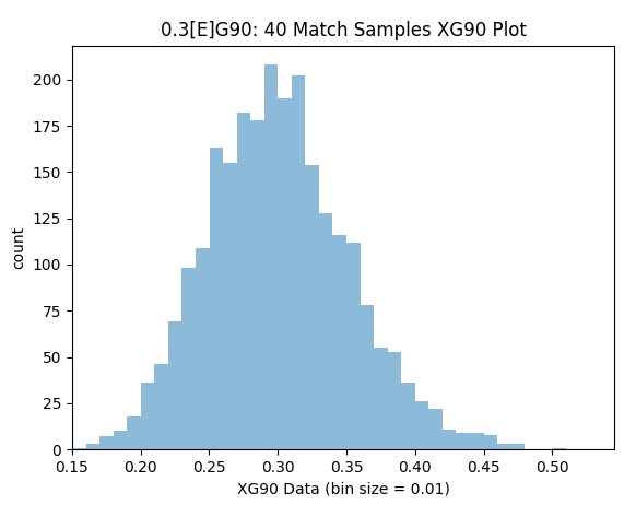
Samples within 10% Precision (0.275-0.325): 44.6%
Samples within 25% Precision (0.225-0.375): 85.4%
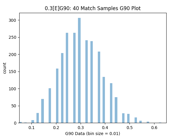
Samples within 10% Precision (0.275-0.325): 32.4%
Samples within 25% Precision (0.225-0.375): 68.9%
*Note my reference to error is not an indication that the xG90 data is wrong, for what it does (ie. describing the quality of shots a player took) it can be considered correct but using it to infer predictive goalscoring potential creates an error as that is not what xG90 data really does.
How Does this Simulation Relate to Real Life Data?
Creating a fancy pants simulation with a ‘perfect shot-based xG model’ is all well and good but does this actually reflect reality where we only have existing non-perfect shot based xG models (though I do think they are very good!) and we do not know a players exact goalscoring potential and can only estimate?
This can just about be investigated but requires the use of an assumption for a players goalscoring potential [E]G90 value. Fortunately Implied Odds data can act in this role as a very good but again imperfect source.
From the 2018/2019 Premier League Season I have 247 samples of players who played 90 minutes with pre-match Implied Odds Goals (ioG) in the range of 0.26-0.35ioG. The mean ioG across the sample was 0.2985ioG.
I have both the post-match Understat xG data and the actual goals scored for each sample too which allows for the same analysis to be run for the 1 match samples (unfortunately there’s not enough data to really extend to 5+ match sequences). I show the actual match-level Understat xG data for this sample below.
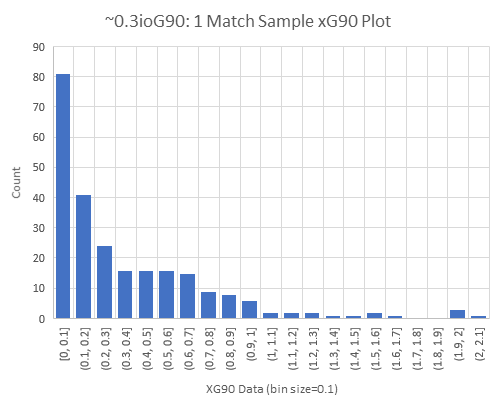
Samples within 10% Precision (0.275-0.325): 3.2%
Samples within 25% Precision (0.225-0.375): 10.5%
This data is very much in line with was expected. It is a degraded version of the perfect xG simulation (which is to be expected as there is no real-life perfect xG model). It is still massively better than the results from basic goal data and it should be noted that in this case the value xG data is likely underestimated as a very good but imperfect source (ioG) is being used for [E]G90. So in reality the margin of error is likely somewhere between the simulation and this estimation from the 247 samples.
I show the simulated results below, which is 100,000 match samples using the perfect xG model and it really matches up well with the real values (which suffers from being a fairly small sample).
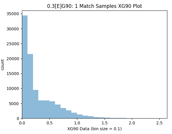
Samples within 10% Precision (0.275-0.325): 4.0%
Samples within 25% Precision (0.225-0.375): 10.9%
Another interesting note is that the goals scored by the players in the real 247 ~0.3 ioG sample fits a Poisson distribution extremely well. 73.3% of the time the player didn’t score, 74.1% is the value expected from a Poisson distribution. 23.1% of the samples scored 1 goal, 22.2% expected from a Poisson distribution. 3.6% of the samples scored 2 goals, 3.3% expected from a Poisson distribution.
That’s not Real-World Enough. Prove it More!
A more straightforward experiment can be performed by using the Understat 2018/2019 EPL data and contrasting a players xG90 from the first half of the season with their xG90 value from the second half of the season.
To create a usable sample I limited the data to players who played at least 900 minutes of football in the first and second half of the season. I also filtered the sample to players who average scored 0.2 and 0.4xG90 in the first half of the season so it can relate to the analysis performed so far. What remained was 20 players who on average played the equivalent of 15 matches in both parts of the season with a mean xG90 of 0.318 in the first 19GWs.
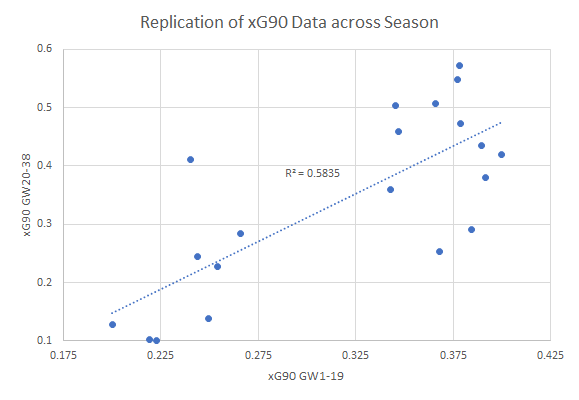
xG90 (20-38) within 10% Precision of xG90 (1-19) : 25.0%
xG90 (20-38) within 25% Precision of xG90 (1-19) : 45.0%
As the graph above shows xG90 is valuable and a great general brushstroke concept of determining a players goalscoring ability.
In terms of this analysis the numbers are extremely strong. The precision indicators from the on average 15 game real world xG model line up almost perfectly with what the perfect xG simulation achieved in 10 game sequences. Remember a real-world xG model is expected to take longer to achieve the kind of accuracy found with the perfect simulated model.
Replication with 10% precision was achieved 25% of the time with the Understat data compared to 22.5% with the simulated 10 matches. Replication with 25% precision was achieved 45% of the time with Understat data compared to 52.7% of the time with the simulated data. The MAE and RMSE of the Understat data was 0.090 & 0.108 which relates very well to 0.0827 & 0.104 in the 10 match sequence simulations.
How well these tests match up with the expectations driven by these simulations appears to be a very strong validation.
Do High Goalscoring Potential Players Converge Faster?
The next question is whether the precision of xG90 data changes with higher [E]G90 players. For this the analysis is repeated to find the xG90 readings for 0.10 & 0.60 [E]G90 players over 40 matches.
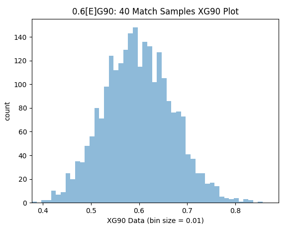
Samples within 10% Precision (0.54-0.66): 59.4%
Samples within 25% Precision (0.45-0.75): 96.7%
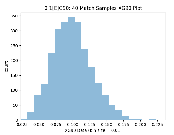
Samples within 10% Precision (0.09-0.11): 28.1%
Samples within 25% Precision (0.075-0.125): 61.6%
The results here are quite intuitive. We can have more confidence in the data for players who get more chances, simply because there are more samples over the same time period. So for players like Aguero or Kane after 40 matches we can have more relative confidence in their xG90 reading compared to defence minded players like Kante.
How About Team Level xG data?
As seen the greater volume of sample- the greater the confidence level we can have in the data. We could assume a typical team is equivalent to 1.40[E]G90 and repeat the process.
Interestingly even at team level 5 matches is still distorted and quite imprecise with regard to the teams true goalscoring potential level as shown below.
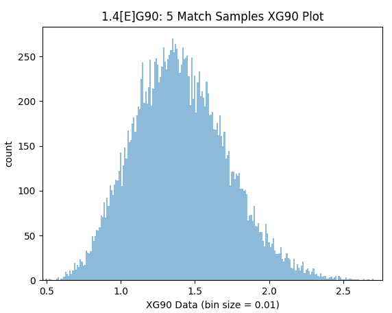
Samples within 10% Precision (1.26-1.54): 33.5%
Samples within 25% Precision (1.05-1.75): 72.9%
However after 40 games we can have very high confidence in the Team Level xG90 data measurements (MAE 0.089 [6.4%], RMSE 0.111, 10% Precision 79.7% of the time, 25% Precision 99.7% of the time). It’s worth noting that it would take 150-200 matches to get the same confidence in the data for a player such as Kevin De Bruyne- which hopefully put’s in perspective how useful xG data is can be at team level.
Why is There Still Significant Variance?
Shot based xG data improves upon basic goal and shot data as it provides more context to an event. Typically it will use key pieces of info from the shot such as: the previous action(s), shot location, body part used, big chance info etc.
This added context reduces variance very significantly but the full picture is still not provided. Consider the following two situations:
- D. Duff makes a tremendously timed run between the centre-halves and will be straight through on goal if his team-mate can complete an extremely straight-forward unmissable pass. Unfortunately his team-mate attempts an unnecessary rabona and trips over the ball.
- Following a corner kick the ball is scrappily being pinged around the penalty area before falling to G. Breen one yard from the goal who was slow to head back towards the half way line as he had been telling a tasteless joke to the opposition goalkeeper.
In those scenarios Duff had a 90% chance of getting at least a reasonably high xG chance but left with 0.00xG and Breen might have had a 0.1% chance of getting such a high xG chance. Of course this is extreme and over enough time it does balance out significantly and this exact problem exists with shot & goal data too. But it does help explain why we need to be careful when looking at low samples of xG data.
And while a full context xG model is just a pipe dream the concept is worth understanding. In reality for each attacking movement every player has a changeable associated % chance of scoring at every point in time as the attack progresses based on the permutations of what could happen next. Also for every shot taken there was only a small fraction of a chance that the specific situation would have occurred at the root of the attack. You could anticipate that there would remain a level of variance with even that model and until things advance to that ridiculous level shot-based xG data remains a fantastic advance.
Conclusion
So having read all the way down here it’s about time I get to the point, how many match samples are required for a useful xG90 reading? Is xG90 data useful? Well it depends… Anything less than 10 matches has incredible potential for distortion and I’d advise caution reading to much into it in isolation at a player-level. 100 matches likely contains outdated data but is a nice reference point. It would seem that the past season or ~40 previous matches would be a safe pick if you want to keep it simple and don’t see reason why it wouldn’t be replicated.
A smart model might look at all past seasons, giving higher weightings to fresher & greater sample data while giving reference to the team quality & the players role (position and set-piece hierarchy) in the team at the time- and then consider the players current situation. It might also refresh after each and every match to maintain a live rating- though that is really for people who want to spend significant time on this.
In terms of how accurate we can expect xG90 data to be for an ~0.3[E]G player the mean error was 13.7% using the perfect xG model over 40 matches, we may expect this to be ~15+% with a real life xG model. For a ~0.6[E]G90 player this was 9.7% with the perfect model but may be more like ~12.5% with a real model. For a ~0.10[E]G90 player the mean error can be expected to be ~25-30% over 40 matches.
But there is an added difficulty here. What we are truly interested in determining is what the player goalscoring potential is going to be over a future set of matches not his past set-point, for the this there is better context to be found in the last 5 matches. I’m not referring to xG data but more a more holistic sense of what role a player is playing, how he is fitting into the team and if his extra-marital affair is going well lately.
The idea that we could predict every players real live goalscoring potential within anything beyond 5% is likely folly, so I hope people do not get disheartened by the numbers described above- well handled xG90 data remains valuable as a predictive measure (more to come on this in my next analysis).
Overall it has to be said that actually watching matches with your very own eyeballs is a good idea too, and can help determine a players true goalscoring potential particularly if you interested in a specific few players and can think things through analytically. Noticing that T. Cascarino was getting into promising positions but didn’t quite get the service he deserved is valuable. Unfortunately highlights miss tonnes of context but are still also very useful- indeed you are likely to run into similiar issues and conclusions as are found with xG data. Though trying to determine proper goalscoring potentials for all 500+ players would be a full-time job and would kill the fun from watching football, not to mention any improvement would definitely be marginal compared to a good model. So the info from xG models remains invaluable when used well and in conjunction with other information sources.
One of those other powerful sources for determining goalscoring potential is Implied Odds Data. This is what is used in the Team Planner tool and in the coming weeks I will be releasing an analysis of the predictivity of Implied Odds data in 2018/19 and will be comparing it to a mathematically perfect model and also a predictive model impregnated with errors similiar to what has been found in this analysis of xG90 data.
Congratulations to anyone who has made it all the way down here- I hope you gained something useful from it!